Explore a Git Repo with R

To better understand how complex software projects are evolving it can be helpful to evaluate the associated Git repo. In this post I'll go over how to retrieve a Git repo and perform various analysis on it using R.

All of these exercises were done within an R notebook in RStudio. You can use any IDE you wish.

Load libraries

First, we'll install the following libraries.

``
library(tidyverse)
library(glue)
library(stringr)

Clone a repo

The first thing we want to do is clone a Git repo onto our local device. This gives us complete control over the repo without needing to worry about impacting anyone. We'll evaluate the ggplot2 repository, just for fun.

First, define where the repo is located.

``
# Remote repository URL
repo_url <- "https://github.com/tidyverse/ggplot2.git"

Then let's create a directory into which the repo will be cloned. The tempdir() command is an easy way to set up a temporary directory.

``
clone_dir <- file.path(tempdir(), "git_repo")

Create the command that will clone the repo to your local machine.

`
clone_cmd <- glue("git clone {repo_url} {clone_dir}")

And invoke the command. Note that this might take while, depending on the size of the repo. Don't freak out, be patient, everything is going to be fine.

``
system(clone_cmd)

When the clone is complete, check that all is well by looking at the git logs. The next line grabs the first three entries of the repo log.

``
system(glue('git -C {clone_dir} log -3'))

In their raw form, logs are pretty messy. We can tidy them up using the pretty format options available in git:

`
log_format_options <- c(datetime = "cd", commit = "h", parents = "p", author = "an", subject = "s")
option_delim <- "\t"
log_format   <- glue("%{log_format_options}") %>% glue_collapse(option_delim)
log_options  <- glue('--pretty=format:"{log_format}" --date=format:"%Y-%m-%d %H:%M:%S"')
log_cmd      <- glue('git -C {clone_dir} log {log_options}')
log_cmd

Now let's look at the logs once again

``
system(glue('{log_cmd} -3'))

That's better.

Time to explore a little. First we can look at the history of commits.

``
history_logs <- system(log_cmd, intern = TRUE) %>%
  str_split_fixed(option_delim, length(log_format_options)) %>%
  as_tibble() %>%
  setNames(names(log_format_options))

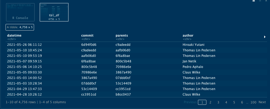
history_logs

A tibble will be produced containing the commit history, looking something like this:

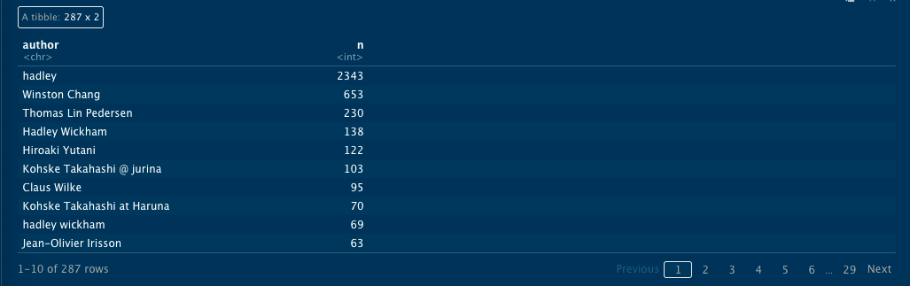
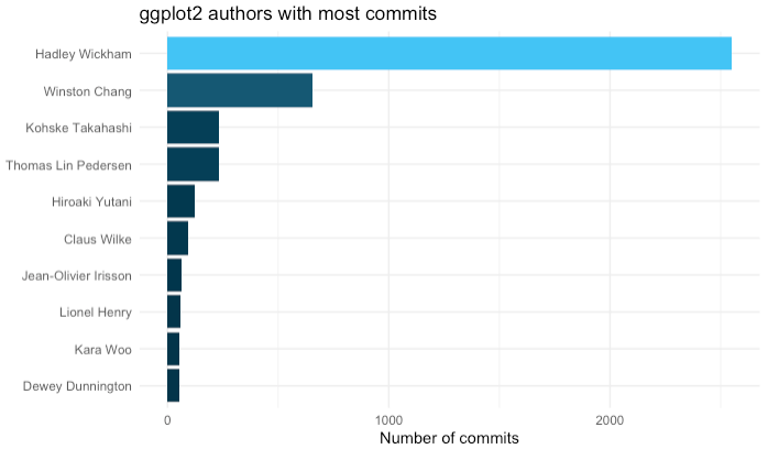
Let's take a look at who is doing most of the work in this repo.

`
history_logs %>%
  count(author, sort = TRUE)

Tidy author names

It's common in Git repos for the same author to use different names. This usually happens when people log in from different computers. In this case you see that there are three variations of Hadley Wickham, including "hadley," "hadley wickham" (lower case), and "Hadley Wickham" (upper case). Let's clean these up.

``
history_logs <- history_logs %>%
  mutate(author = case_when(
    str_detect(tolower(author), "hadley") ~ "Hadley Wickham",
    str_detect(tolower(author), "kohske takahashi") ~ "Kohske Takahashi",
    TRUE ~ str_to_title(author)
  ))

Graph authors

And now we can visualize the authors using ggplot

``
history_logs %>%
  count(author) %>%
  top_n(10, n) %>%
  mutate(author = fct_reorder(author, n)) %>%
  ggplot(aes(author, n)) +
    geom_col(aes(fill = n), show.legend = FALSE) +
    coord_flip() +
    theme_minimal() +
    ggtitle("ggplot2 authors with most commits") +
    labs(x = NULL, y = "Number of commits")

Visualize directories

We cloned the git repo into a temporary directory. Now we are able to perform certain git commands and understand commits etc. Now we'll explore the file directory. To do that we need to create a tibble out of the file directory. You might remember that our repo is located at the variable clonedir

We'll use the fs library to create the first tibble of the directory, with path type and size.

``
library(fs)
repofiles <- dir_info(clone_dir, recurse = TRUE) %>% select(path, type, size) %>% group_by(path)

This will create a tibble that contains all the temporary directories. We don't care about those, so let's tidy up a bit by getting rid of them. (Note that your path will differ from mine, you should replace the string with the path that was actually created on your machine).

``
 repofiles <- repofiles %>% mutate(path = str_remove(path, "/var/folders/n0/13y4pg1d20l4th9zbqpzjd640000gr/T/Rtmp1i69Wg/"))

The tibble contains both directories and files. Let's split the two so we don't get confused about what kind of data is contained where.

``
repodir <- filter(repofiles, type == "directory")

repofiles <- filter(repofiles, type == "file")

The visualization we'll use is looking for a column called pathString, so lets create it

``
repofiles$pathString <- repofiles$path

Just for fun, let's also split out all the directories into their own columns.

``
repofiles <- separate(repofiles, col = "path", c("root", "group", "subgroup", "subsubgroup", "file"), sep = "([/])", fill = "right")

The visualization engine needs the data to be in node format, so let's create that

``
repoviz <- as.Node(mytree_file)

Let's install the libraries we'll need. You might need to install the circlepackeR library first. It's not on CRAN, so grab it from Github instead

``
devtools::install_github("jeromefroe/circlepackeR")

Then load the library

``
library(circlepackeR)

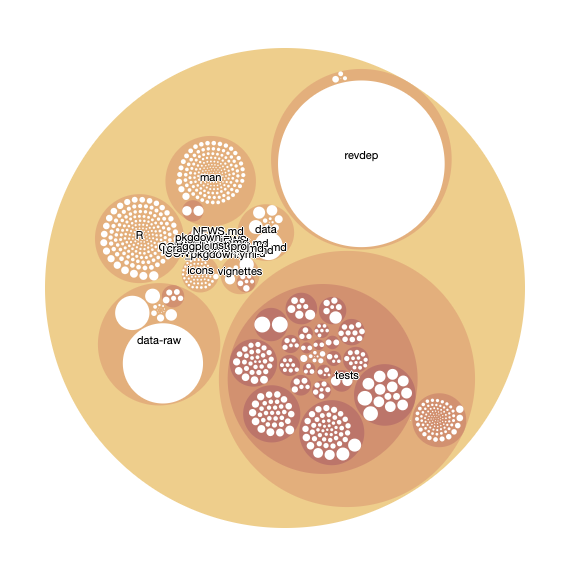
Create the visualization

``
circles <- circlepackeR(repoviz, size = "size", color_min = "hsl(56,80%,80%)", color_max = "hsl(341,30%,40%)")

And save it so that you can interact with it.

``
library(htmlwidgets)
saveWidget(circles, file=paste0( getwd(), "/HtmlWidget/circular_packing_circlepackeR2.html"))

The file will appear in RStudio under the "files" section.

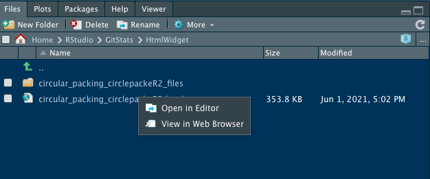
And there you have it!